PoleClinometer® Math
Want to dig in and understand exactly what defines those funny curved lines that allow a PoleClinometer sticker to do its thing? Here’s the detailed math behind the magic.
Cartesian & Cylindrical Coordinates
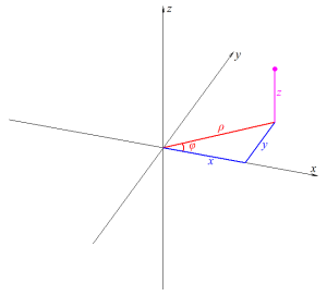 We’ll use both Cartesian & Cylindrical 3D coordinate systems here, so let’s start by identifying some simple conversions between the two. We’ll use the numbered equations later.
Cylinder & Plane
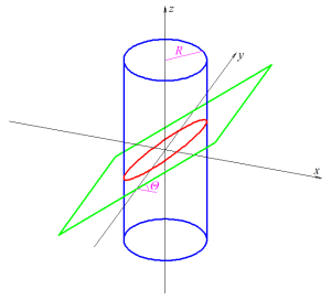 Now let’s define a vertical cylinder of radius R, centered about the z axis (illustrated in blue here). The equation for the surface of that cylinder in Cartesian coordinates, is:
Applying eq.2 (or common sense), the equation for this cylinder in Cylindrical coordinates is simply:
Now let’s define a plane containing the y axis, and at an angle of Θ to the x axis (illustrated in green here). The equation for that plane, in Cartesian coordinates, is:
Applying eq.1, the equation for this plane in Cylindrical coordinates is:
Combine eq.3 (the cylinder) and eq.4 (the plane) to solve for the intersection of the surface of the cylinder with the plane (illustrated in red here), expressed in Cylindrical coordinates:
So that’s the equation for a PoleClinometer line in 3D space with the sticker applied to a ski pole shaft, where Θ is the slope angle represented by the line, and R is the radius of the pole shaft. Now the trick is to determine the equation for that line in 2D space on the surface of the sticker when it’s “unwrapped” from the shaft of the ski pole. This turns out to be a pretty simple geometric transformation, especially with our equation in 3D space already represented in Cylindrical coordinates.
“Unwrap” Geometric Transformation
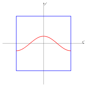 To quantify our slope line as plotted on a 2-dimensional sticker, we need to create a new 2D space to work in. Let’s call our new 2D coordinates x’ and y’ to distinguish the 2D “unwrapped” sticker space from the x,y,z or ρ,φ,z of the 3D space we’ve been working in.
We know the circumference of the cylinder is:
And of course the width of the sticker (in the new x’ dimension) is equal to the circumference of the cylinder (i.e. we want the sticker width to be such that the edges just meet when we wrap it around the pole shaft). So a range of φ from 0 to 2π (i.e. a 360° swing around the surface of the cylinder) maps linearly to a range of x’ from 0 to C (i.e. the full width of the sticker). That says x’ can be expressed as:
Solving for φ we get:
And our new y’ maps directly from the z of our 3D space, so from eq.5 and eq.7 we have:
Expressing this in terms of circumference rather than radius (per eq.6) we get:
Offset for Multiple Lines
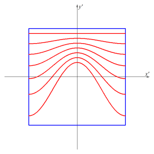 Since we want to plot multiple lines on one sticker, each representing a unique slope angle, we can simply add an arbitrary offset unique to each line to keep them suitably spaced apart:
Each line will have a unique value of Θ for a specific slope angle, and a unique value of A to keep the lines from running into one another.
Note that the range of x’ over which the lines are plotted determines where the “break” in the sticker is. To align the break in the sticker with the bottom of the sinusoidal curves, PoleClinometer sticker lines are plotted over the range –C/2 to +C/2. So representing this explicitly in the eqution we get:
So there you have the equation for those magical slope lines on a PoleClinometer sticker. Who ever said math wasn’t fun and practical?
😎
